microbetag on Cytoscape
Run microbetag Cytoscape app
All you need to do for start using microetag is first, to download Cytoscape in case not already on your computer, and then install the microbetag app (MGG) from Cytoscape App store. If you visit Cytoscape Appstore and you have not lunched Cytoscape, you will see a Download button. Please, make sure you first lunch Cytoscape and then visit Cytoscape, otherwise, lunch Cytoscape and refresh the Cytoscape Appstore page. Now, you will see that the Download button has turned to Install. By clicking it, it will be automatically integrated on your Cytoscape. This can also be performed from within Cytoscape by clicking on the Apps tab of the main bar and then App Store > Show App Store and typing microbetag on the box that pops up.
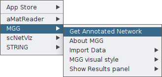
Once the app is installed, you may click on the Apps tab and you will find MGG there.
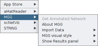
From this box, you will have access to all features of the app. As you see, the Get Annotated Network is currently not a clickable option. That is because microbetag has no input yet.
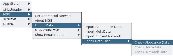
You need first to feed the app with your abundance table and, if available, your co-occurrence network. In both cases though, the abundance table will be required and this is why when you click on Import Data you currently see only the Import Abundance Data option.
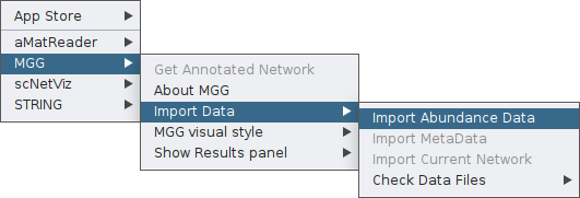
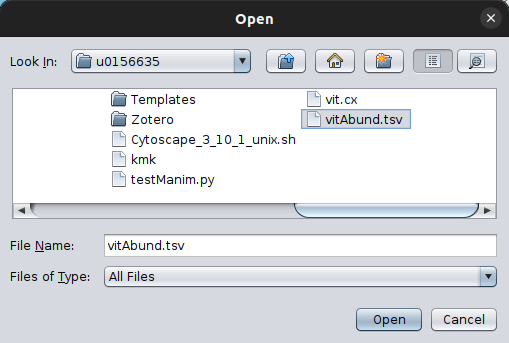
By clicking on it, a pop-up box will ask you to provide your abundance table. In this example, we will use the vitAbund.tsv file. Select it whith you mouse and then open it.
To make sure of the imported data, you can then check them, using the corresponding option from the Check Data Files feature, in this case the abundance tabe:
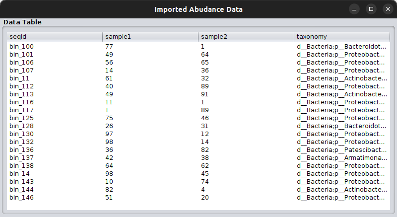
Once clicking that, a table will pop up where you can go through the data you have imported as the abundance table.
Please, make sure your taxonomy fits the criteria for microbetag to run. You may find more on that issue on the Input files section.
Then, as you will see in the following two cases, you will have to set the values to a set of parameters to describe your input data but also what annotation steps you would like microbetag to perform.
| Variable | Description | Value |
|---|---|---|
input_category | In case you already have a network, set it as network and load it; otherwise set it as abundance_table. In both cases you need to provide the abundance table though | abundance_table | network |
taxonomy | In case a user’s taxonomy is to be used, denotes which taxonomy scheme to be used from microbetag | [GTDB | dada2 | qiime2] |
phenDB | return phenotypic traits based on phen models | bool |
faprotax | return annotations using the FAPROTAX database | bool |
pathway_complement | return pathway complmementarities between associated nodes | bool |
seed_scores | return complementarity and cooperation scores based on metabolic reconstructions seed sets | bool |
manta | return clusters of nodes on the network using the manta package | bool |
get_children | use genomes of children taxa of the taxa in the abundance table based on the NCBI Taxonomy scheme | bool |
heterogeneous | (FlashWeave) enable heterogeneous mode for multi-habitat or -protocol data with at least thousands of samples (FlashWeaveHE) | bool |
sensitive | (FlashWeave) enable fine-grained associations (FlashWeave-S, FlashWeaveHE-S), sensitive=false results in the fast modes FlashWeave-F or FlashWeaveHE-F | bool |
.. starting from an abundance table
In this case, microbetag can come up with a co-occurrence network using FlashWeave. The on-the fly creation of the co-occurrence network is supported only for abundance tables with up to 1000 records.
Once your abundance table is imported, you can now ask for a microbetag-annotated network by clicking on the corresponding feature:
Once clicking on that, a parameter-setting box will pop-up, asking for values on a number of parameters essential for the successful network inference and their corresponding annotation.
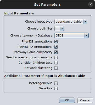
Please make sure you set the input type as abundance_table and you select the correct taxonomy scheme. It is crucial to also set the FlashWeave related parameters in a way they address your abundance table idiosyncracy.
We suggest you do the network inference step as well as the mapping to the GTDB taxonomy before using microbetag through the Cytoscape App as this would provide you extra freedom on they network inference and gain dramatically in computing time on the server.
Once you set the parameters of your choice, you are ready to sent your query to the server by clicking ok.
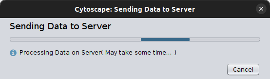
After a few minutes (based on your data and the steps you have asked for) a microbetag-annotated network will pop up automatically on your Cytoscape instance.
UP LIMIT FOR ABUNDANCE TABLE RECORDS
microbetag will build a co-occurrence network only for abundance tables with less than 1000 of records. In case your abundance table is larger, you will have to run the microbetag prepropcess steps. Otherwise, you can always run any algorithm for network inference locally and use their findings with microrbetag.
.. starting from a co-occurrence network
If you already have a network, then you need to provide both the network and the abundance table and make sure that the sequence identifiers in those two files are the same; meaning that the node ids of the network are present in the abundance table in the column representing the sequence identifier.
For example, a toy model of a network file would be:
| node_A | node_B | weight |
|---|---|---|
| bin_1 | bin_2 | 0.84 |
then, the corresponding abundance table would have, among other records, to have the following two lines:
| sequenceIdentifier | sample_1 | sample_2 | sample_3 | taxonomy |
|---|---|---|---|---|
| bin_1 | 234 | 42 | 43 | g__Devosia;s__Devosia sp001899045 |
| bin_2 | 324 | 54 | 43 | g__Pseudonocardia;s__Pseudonocardia sp001899645 |
Taxonomy here is only partial. Make sure you always have a 7-level taxonomy, e.g. d__Bacteria;p__Proteobacteria;c__Alphaproteobacteria;o__Rhizobiales;f__Devosiaceae;g__Devosia_A;s__Devosia_A sp001899075
Once you are sure of these requirements, you can import your network through the main File tab of Cytoscape:
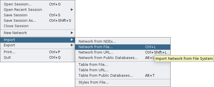
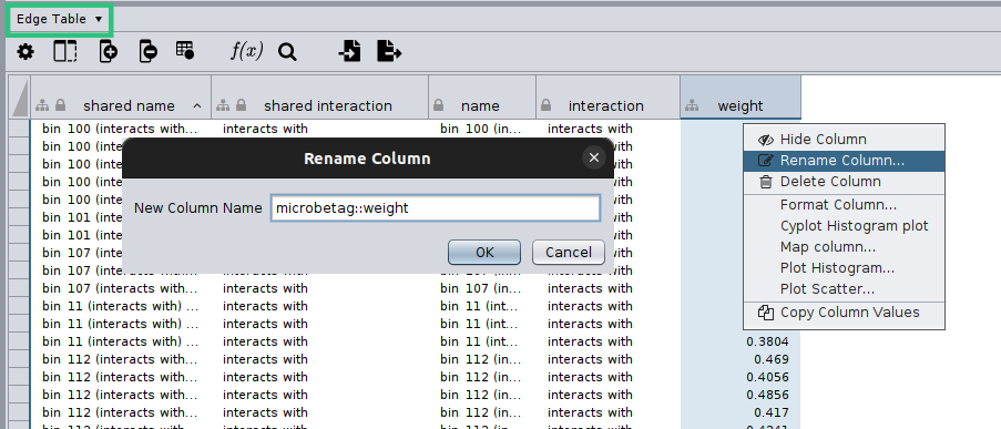
Cytoscape will display your network and on the bottom of your screen you will have the core tables of a Cytoscape network. As your network may have several edges, you need to make clear which edge attribute you would like microbetag to use; this is essential in cases network clustering will be performed. To do so, you need to move on the Edge table by clicking on the arrow next to the Node table that is displayed by default, and then remame the column of your choice to microbetag::weight.
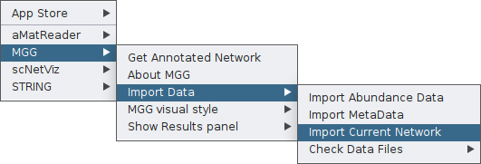
Now you are ready to import your network to MGG though its main menu on the Apps tab:
Finally, you can again check your network as loaded on MGG through the Check Data Files tab:
If the node names of the network are not included in the sequence identifiers of the abundance table, you will not be able to import your network to MGG.
Once both your abundance file and your network are imported, you can proceed as in the Starting from an abundance table case by clicking on Get Annotated Network on the main menu of the MGG app on the Apps tab and setting the parameters required.
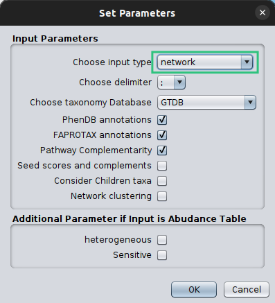
Make sure that you set the Choose Input Type as network this time, otherwise microbetag will ignore your network and try to build on of their own.
“Roaming” acrross annotated nodes and edges
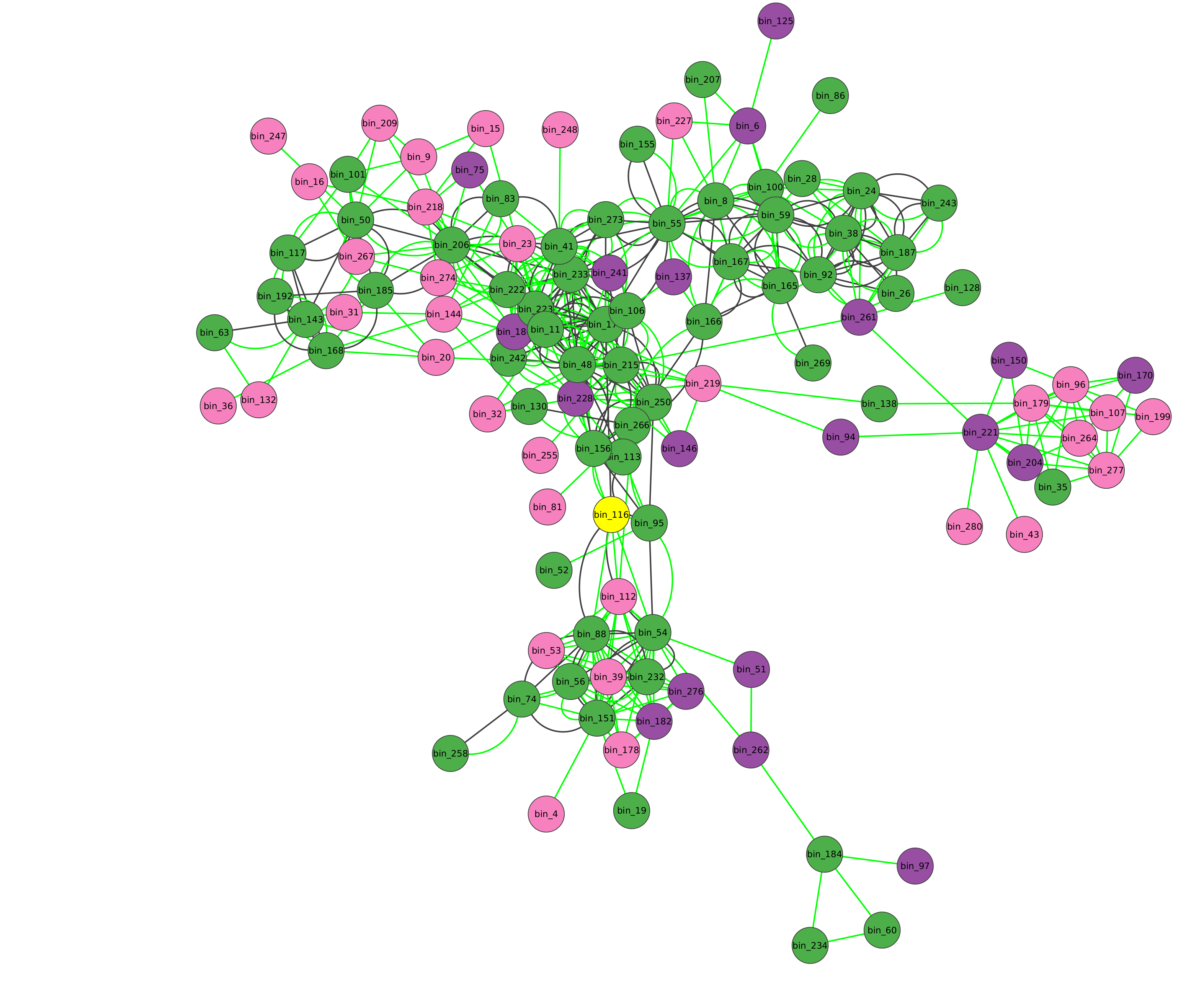
Once an annotated network is returned (or loaded), you have all Cytoscape features (e.g., annotation, filtering, selecting etc.) plus those coming from the microbetag App facilitating a user-friendly way to go through the annotations returend.
Color-coding of the nodes (taxa) denoted the taxonomic level that a certain sequence was able to be mapped on microbetag.
green
node was mapped to a genome (i.e. species/strain) and annotations are available for it
pink
node was mapped to the genus level; annotations limited to literature-oriented (FAPROTAX)
purple
node was mapped to the family level; likewise, only FAPROTAX annotations occasionaly
red
node was mapped to higher taxonomic level and no annotations were returned
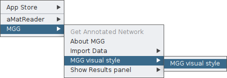
If you edit the style of your microbetag-annotated network, you can always bring back its original style through the MGG main menu.
By clicking on the Show Species button, all nodes that were not mapped to a genome will be masked.
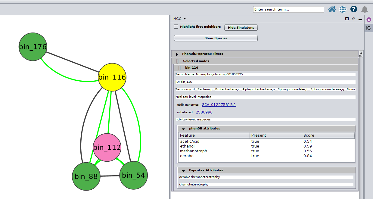
Or you can choose/click directly any node on the network and check the Nodes Panel
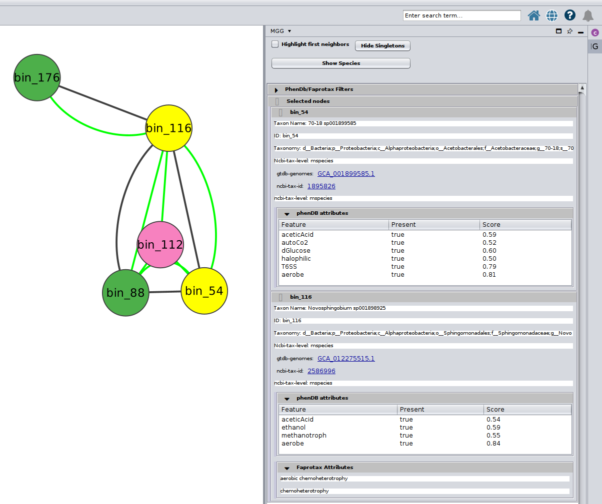
or several at the same time
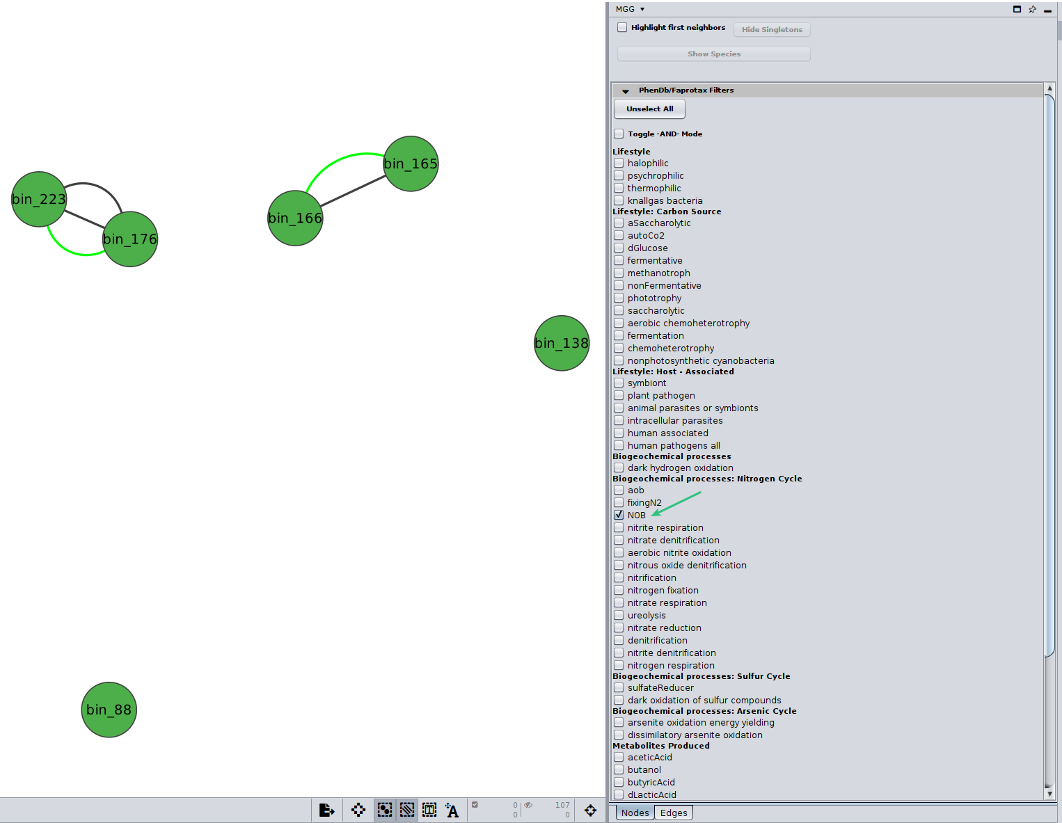
Further, you may selecet among a list of annotations under the PhenDb/FAPROTAX filters with AND and OR relationships. For example, I was curios about the Nitrite-oxidizing bacteria (NOB) on my network
Likewise, you may go through the annotations on the edges of the network.
Edges are either
green
mentioning co-occurrences
red
suggesting mutual exclusion of the two taxa
black
representing directed potential metabolic interactions.
One may select from the two top buttons on the Edges panel to show only edges with pathwawy complementarities or seed complementarities.
By clinking on a potential metabolic interaction edge, the donor and the beneficiary species, along with their corresponding sequence identifiers will be displayed highlighting who potentially benefits from the other.
Then, for cases where pathway complementarities have been returned for this association, a panel will be available for each pair of genomes that were mapped to those two taxa. For each pair of genomes, a list with the potential metabolic complementarities is then returned. In the first column the KEGG MODULE id of the corresponding complementarity is provided, and in the second and third column their description and metabolism category. In the fourth column, called “Complement” the KO that need to be provided to the beneficiary species to support the module are given and in the next column, the complete alternative that would then faciliate the module is shown; i.e., assuming the complement is provided.
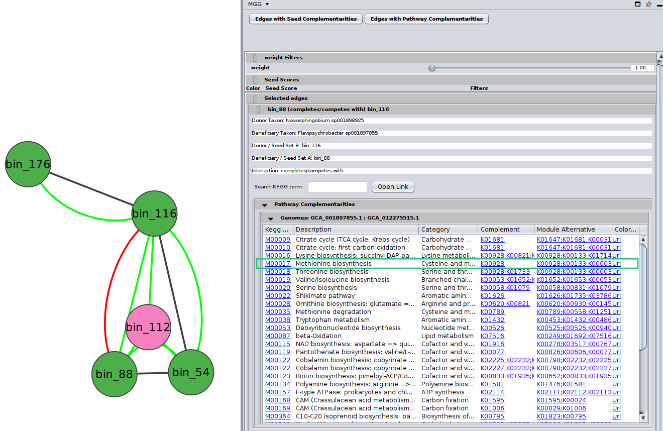
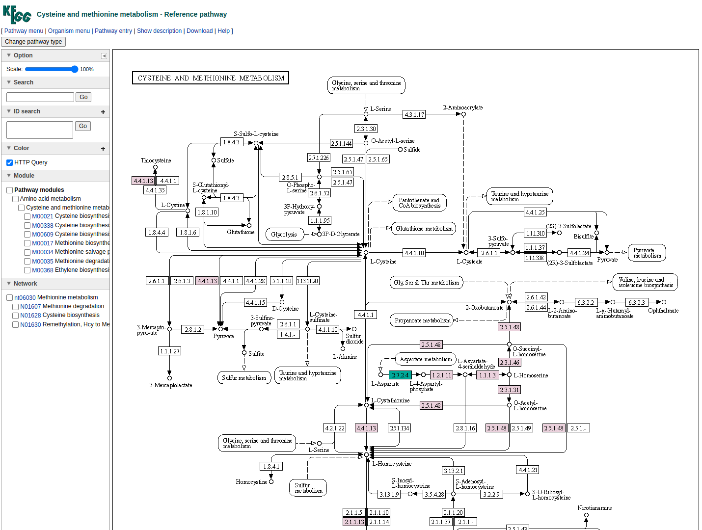
In the final column a link to a related KEGG map is provided where KO available in the beneficiary species are colored with pink and those provided by the donor in the scenario of the potential metabolic interaction with green. The screenshot below illustrates the highlighted complementarity in the biosynthesis of methionine.
Moerover, microbetag may also return seed complements. Like in the case of the patwhay complementarities, a new panel is displayed when seed complements are available for an edge. Here is an example:
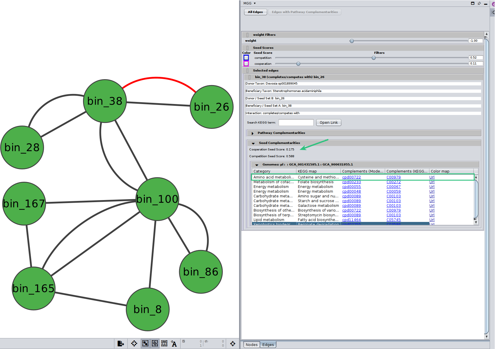
Seed scores between the two genomes are also shown here. Remebmer that like the edge under study, seed scores have also directionality; seed score for competiotion between $genome_A$ and $genome_B$ is not necessarily the same with the one between $genome_B$ and $genome_A$. Those scores are only indicative and they should not be considered as fact of observed cooperation/competition. Seed complements are then recorded in the same way as pathway complementarities. However, there is no Complement column as this time it is not a specific KEGG MODULE that is supported, rather a potential range of functions that can be viewer through the colored url. Also, a new column provides the ModelSEED compound id that was actually found as a complement and was then mapped to their KEGG corresponding one.